Table of Contents
Introduction
Now that we are ready to start working with Canadian Census data, let’s first briefly address the question why you may need it. After all, CANSIM data is often more up-to-date and covers a much broader range of topics than the national census data, which is gathered every five years in respect of a limited number of questions.
The main reason is that CANSIM data is far less granular geographically. Most of it is collected at the provincial or even higher regional level. You may be able to find CANSIM data on a limited number of questions for some of the country’s largest metropolitan areas, but if you need the data for a specific census division, city, town, or village, you’ll have to use the Census.
To illustrate the use of the cancensus package, let’s do a small research project. First, in this post we’ll retrieve the following key labor force characteristics of the largest metropolitan areas in each of the five geographic regions of Canada:
- Labor force participation rate, employment rate, and unemployment rate.
- Percent of workers by work situation: full time vs part time, by gender.
- Education levels of people aged 25 to 64, by gender.
The cities (metropolitan areas) that we are going to look at, are: Calgary, Halifax, Toronto, Vancouver, and Whitehorse. We’ll also get these data for Canada as a whole for comparison and to illustrate the retrieval of data at different geographic levels
Next, in Part 6 of the “Working with Statistics Canada Data in R” series, we will visualize these data, including making a faceted plot and writing a function to automate repetitive plotting tasks.
Keep in mind that cancensus also allows you to retrieve geospatial data, that is, borders of census regions at various geographic levels, in sp and sf formats. Retrieving and visualizing Statistics Canada geospatial data will be covered later in these series.
So, let’s get started by loading the required packages:
Searching for Data
cancensus retrieves census data with the get_census() function. get_census() can take a number of arguments, the most important of which are dataset, regions, and vectors, which have no defaults. Thus, in order to be able to retrieve census data, you’ll first need to figure out:
- your dataset,
- your region(s), and
- your data vector(s).
Find Census Datasets
Let’s see which census datasets are available through the CensusMapper API:
Currently, datasets earlier than 1996 are not available, so if you need to work with pre-1996 census data, you won’t be able to retrieve it with cancensus.
Find Census Regions
Next, let’s find the regions that we’ll be getting the data for. To search for census regions, use the search_census_regions() function.
Let’s take a look at what region search returns for Toronto. Note that cancensus functions return their output as dataframes, making it is easy to subset. Here I limited the output to the most relevant columns to make sure it fits on screen. You can run the code without [c(1:5, 8)] to see all of it.
# all census levels
search_census_regions(searchterm = "Toronto",
                      dataset = "CA16")[c(1:5, 8)]

#> # A tibble: 3 x 6
#>   region  name    level     pop municipal_status PR_UID
#>   <chr>   <chr>   <chr>   <int> <chr>            <chr>
#> 1 35535   Toronto CMA   5928040 B                35
#> 2 3520    Toronto CD    2731571 CDR              35
#> 3 3520005 Toronto CSD   2731571 C                35
You may have expected to get only one region: the city of Toronto, but instead you got three! So, what is the difference? Look at the column level for the answer. Often, the same geographic region can be represented by several census levels, as is the case here. There are three levels for Toronto, which is simultaneously a census metropolitan area, a census division, and a census sub-division. Note also the PR_UID column that contains numeric codes for Canada’s provinces and territories. These codes can help you distinguish between different census regions that have same or similar names but are located in different provinces. For an example, run the code above replacing “Toronto” with “Windsor”.
Remember that we were going to plot the data for census metropolitan areas? You can choose the geographic level with the level argument, which can take the following values: ‘C’ for Canada (national level), ‘PR’ for province, ‘CMA’ for census metropolitan area, ‘CD’ for census division, ‘CSD’ for census sub-division, or NA:
# specific census level
search_census_regions("Toronto", "CA16", level = "CMA")
Let’s now list census regions that may be relevant for our project:
# explore available census regions
names <- c("Canada", "Calgary", "Halifax",
           "Toronto", "Vancouver", "Whitehorse")
map_df(names, ~ search_census_regions(., dataset = "CA16"))[c(1:5, 8)]

#> # A tibble: 19 x 6
#>    region  name                    level      pop municipal_status PR_UID
#>    <chr>   <chr>                   <chr>    <int> <chr>            <chr>
#>  1 01      Canada                  C     35151728 NA               NA
#>  2 48825   Calgary                 CMA    1392609 B                48
#>  3 4806016 Calgary                 CSD    1239220 CY               48
#>  4 12205   Halifax                 CMA     403390 B                12
#>  5 1209    Halifax                 CD      403390 CTY              12
#>  6 1209034 Halifax                 CSD     403131 RGM              12
#>  7 2432023 Sainte-Sophie-d'Halifax CSD        612 MÉ               24
#>  8 35535   Toronto                 CMA    5928040 B                35
#>  9 3520    Toronto                 CD     2731571 CDR              35
#> 10 3520005 Toronto                 CSD    2731571 C                35
#> 11 59933   Vancouver               CMA    2463431 B                59
#> 12 5915    Greater Vancouver       CD     2463431 RD               59
#> 13 5915022 Vancouver               CSD     631486 CY               59
#> 14 5915046 North Vancouver         CSD      85935 DM               59
#> 15 5915051 North Vancouver         CSD      52898 CY               59
#> 16 5915055 West Vancouver          CSD      42473 DM               59
#> 17 5915020 Greater Vancouver A     CSD      16133 RDA              59
#> 18 6001009 Whitehorse              CSD      25085 CY               60
#> 19 6001060 Whitehorse, Unorganized CSD        326 NO               60
purrr::map_df() function applies search_census_regions() iteratively to each element of the names vector and returns output as a single dataframe. Note also the ~ . syntax. Think of it as the tilde taking each element of names and passing it as an argument to a place indicated by the dot in the search_census_regions() function. You can find more about the tilde-dot syntax here. It may be a good idea to read the whole tutorial: purrr is a super-useful package, but not the easiest to learn, and this tutorial does a great job explaining the basics.
Since there are multiple entries for each search term, we’ll need to choose the results for census metropolitan areas, or in case of Whitehorse, for census sub-division, since Whitehorse is too small to be considered a metropolitan area:
# select only the regions we need: CMAs (and CSD for Whitehorse)
regions <- list_census_regions(dataset = "CA16") %>%
  filter(grepl("Calgary|Halifax|Toronto|Vancouver", name) &
         grepl("CMA", level) |
         grepl("Canada|Whitehorse$", name)) %>%
  as_census_region_list()
Pay attention to how the logical operators are used to filter the output by several conditions at once; also note using $ regex meta-character to choose from the names column the entry ending with ‘Whitehorse’ (to filter out ‘Whitehorse, Unorganized’.
Finally, as_census_region_list() converts list_census_regions() output to a data object of type list that can be passed to the get_census() function as its regions argument.
Find Census Vectors
Canadian census data is made up of individual variables, aka census vectors. Vector number(s) is another argument you need to specify in order to retrieve data with the get_census() function.
cancensus has two functions that allow you to search through census data variables: list_census_vectors() and search_census_vectors().
list_census_vectors() returns all available vectors for a given dataset as a single dataframe containing vectors and their descriptions:
# structure of list_census_vectors output
str(list_census_vectors(dataset = 'CA16'))

#> tibble [6,623 × 7] (S3: tbl_df/tbl/data.frame)
#>  $ vector       : chr [1:6623] "v_CA16_401" "v_CA16_402" "v_CA16_403" "v_CA16_404" ...
#>  $ type         : Factor w/ 3 levels "Female","Male",..: 3 3 3 3 3 3 3 3 2 1 ...
#>  $ label        : chr [1:6623] "Population, 2016" "Population, 2011" "Population percentage change, 2011 to 2016" "Total private dwellings" ...
#>  $ units        : Factor w/ 6 levels "Number","Percentage ratio (0.0-1.0)",..: 1 1 1 1 1 4 1 1 1 1 ...
#>  $ parent_vector: chr [1:6623] NA NA NA NA ...
#>  $ aggregation  : chr [1:6623] "Additive" "Additive" "Average of v_CA16_402" "Additive" ...
#>  $ details      : chr [1:6623] "CA 2016 Census; Population and Dwellings; Population, 2016" "CA 2016 Census; Population and Dwellings; Population, 2011" "CA 2016 Census; Population and Dwellings; Population percentage change, 2011 to 2016" "CA 2016 Census; Population and Dwellings; Total private dwellings" ...
#>  - attr(*, "last_updated")= POSIXct[1:1], format: "2020-12-21 23:27:47"
#>  - attr(*, "dataset")= chr "CA16"


# count variables in 'CA16' dataset
nrow(list_census_vectors(dataset = 'CA16'))

#> [1] 6623
As you can see, there are 6623 (as of the time of writing this) variables in the 2016 census dataset, so list_census_vectors() won’t be the most convenient function to find a specific vector. Note however that there are situations (such as when you need to select a lot of vectors at once), in which list_census_vectors() would be appropriate.
Usually it is more convenient to use search_census_vectors() to search for vectors. Just pass the text string of what you are looking for as the searchterm argument. You don’t have to be precise: this function works even if you make a typo or are uncertain about the spelling of your search term.
Let’s now find census data vectors for labor force involvement rates:
# get census data vectors for labor force involvement rates
lf_vectors <-
  search_census_vectors(searchterm = "employment rate",
                        dataset = "CA16") %>%
  union(search_census_vectors("participation rate", "CA16")) %>%
  filter(type == "Total") %>%
  pull(vector)
Let’s take a look at what this code does. Since searchterm doesn’t have to be a precise match, “employment rate” search term retrieves unemployment rate vectors too. In the next line, union() merges dataframes returned by search_census_vectors() into a single dataframe. Note that in this case union() could be substituted with bind_rows(). I recommend using union() in order to avoid data duplication. Next, we choose only the “Total” numbers, since we are not going to plot labor force indicators by gender. Finally, the pull() command extracts a single vector from the dataframe, just like the $ subsetting operator: we need lf_vectors to be a data object of type vector in order to pass it to the vectors argument of the get_census() function.
There is another way to figure out search terms to put inside the search_census_vectors() function: use Statistics Canada online Census Profile tool. It can be used to quickly explore census data as well as to figure out variables’ names (search terms) and their hierarchical structure.
For example, let’s look at the census labor data for Calgary metropolitan area. Scrolling down, you will quickly find the numbers and text labels for full-time and part-time workers:
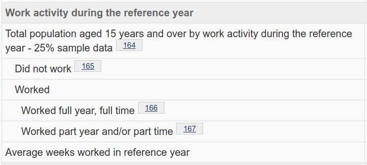
Now we know the exact search terms, so we can get precisely the vectors we need, free from any extraneous data:
# get census data vectors for full- and part-time work
# get vectors and labels
work_vectors_labels <-
  search_census_vectors("full year, full time", "CA16") %>%
  union(search_census_vectors("part year and/or part time", "CA16")) %>%
  filter(type != "Total") %>%
  select(1:3) %>%
  mutate(label = str_remove(label, ".*, |.*and/or ")) %>%
  mutate(type = fct_drop(type)) %>%
  setNames(c("vector", "gender", "type"))

# extract vectors
work_vectors <- work_vectors_labels$vector
Note how this code differs from the code with which we extracted labor force involvement rates: since we need the data to be sub-divided both by the type of work and by gender (hence no “Total” values here), we are creating a dataframe that assigns respective labels to each vector number. This work_vectors_labels dataframe will supply categorical labels to be attached to the data retrieved with get_census().
Also, note these three lines:
  mutate(label = str_remove(label, ".*, |.*and/or ")) %>%
  mutate(type = fct_drop(type)) %>%
  setNames(c("vector", "gender", "type"))
The first mutate() call removes all text up to and including , and and/or (spaces included) from the label column. The second drops unused factor level “Total” – it is a good practice to make sure there are no unused factor levels if you are going to use ggplot2 to plot your data. Finally, setNames() renames variables for convenience.
Finally, let’s retrieve vectors for the education data for the age group from 25 to 64 years, by gender. Before we do this, I’d like to draw your attention to the fact that some of the census data is hierarchical, which means that some variables (census vectors) are included into parent and/or include child variables. It is very important to choose vectors at proper hierarchical levels so that you do not double-count or omit your data.
Education data is a good example of hierarchical data. You can explore data hierarchy using parent_census_vectors() and (child_census_vectors) functions. However, you may find exploring the hierarchy visually to be more convenient:
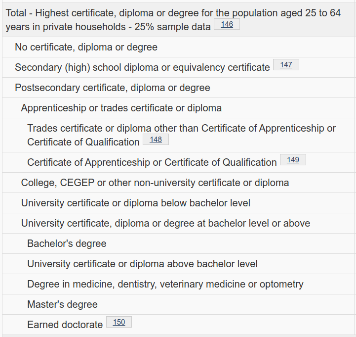
So, let’s now retrieve and label the education data vectors:
# get vectors and labels
ed_vectors_labels <-
  search_census_vectors("certificate", "CA16") %>%
  union(search_census_vectors("degree", "CA16")) %>%
  union(search_census_vectors("doctorate", "CA16")) %>%
  filter(type != "Total") %>%
  filter(grepl("25 to 64 years", details)) %>%
  slice(-1,-2,-7,-8,-11:-14,-19,-20,-23:-28) %>%
  select(1:3) %>%
  mutate(label =
           str_remove_all(label,
                          " cert.*diploma| dipl.*cate|, CEGEP| level|")) %>%
  mutate(label =
           str_replace_all(label,
                           c("No.*" = "None",
                             "Secondary.*" = "High school or equivalent",
                             "other non-university" = "equivalent",
                             "University above" = "Cert. or dipl. above",
                             "medicine.*" = "health**",
                             ".*doctorate$" = "Doctorate*"))) %>%
  mutate(type = fct_drop(type)) %>%
  setNames(c("vector", "gender", "level"))

# extract vectors
ed_vectors <- ed_vectors_labels$vector
Note the slice() function that allows to manually select specific rows from a dataframe: positive numbers choose rows to keep, negative numbers choose rows to drop. I used slice() to drop the hierarchical levels from the data that are either too general or too granular. Note also that I had to edit text strings in the data. Finally, I added asterisks after “Doctorate” and “health”. These are not regex symbols, but actual asterisks that will be used to refer to footnotes in plot captions later on.
Now that we have figured out our dataset, regions, and data vectors (and labeled the vectors, too), we are finally ready to retrieve the data.
Retrieve Census Data
To retrieve census data, feed the dataset, regions, and data vectors into get_census() as its’ respective arguments. Note that get_census() has the use_cache argument (set to TRUE by default), which tells get_census() to retrieve data from cache if available. If there is no cached data, the function will query CensusMapper API for the data and will save it in the cache, while use_cache = FALSE will force get_census() to query the API and update the cache.
# get census data for labor force involvement rates
# feed regions and vectors into get_census()
labor <-
  get_census(dataset = "CA16",
             regions = regions,
             vectors = lf_vectors) %>%
  select(-c(1, 2, 4:7)) %>%
  setNames(c("region", "employment rate",
             "unemployment rate",
             "participation rate")) %>%
  mutate(region = str_remove(region, " (.*)")) %>%
  pivot_longer("employment rate":"participation rate",
               names_to = "indicator",
               values_to = "rate") %>%
  mutate_if(is.character, as_factor)
The select() call drops columns with irrelevant data. setNames() renames columns to remove vector numbers from variable names – we don’t need vector numbers in variable names because variable names will be converted to values in the indicator column. str_remove() inside the mutate() call drops municipal status codes ‘(B)’ and ‘(CY)’ from region names. Finally, mutate_if() line converts characters to factors for subsequent plotting.
An important function here is tidyr::pivot_longer(). It converts the dataframe from wide to long format. It takes three columns: employment rate, unemployment rate, and participation rate, and passes their names as values of the indicator variable, while their numeric values are passed to the rate variable. The reason for conversion is that we are going to plot the data for all three labor force indicators in the same graphic, which makes it necessary to store the indicators as a single factor variable.
Next, let’s retrieve census data about the percent of full time vs part time workers, by gender, and the data about the education levels of people aged 25 to 64, by gender:
# get census data for full-time and part-time work
work <-
  get_census(dataset = "CA16",
             regions = regions,
             vectors = work_vectors) %>%
  select(-c(1, 2, 4:7)) %>%
  rename(region = "Region Name") %>%
  pivot_longer(2:5, names_to = "vector",
                    values_to = "count") %>%
  mutate(region = str_remove(region, " (.*)")) %>%
  mutate(vector = str_remove(vector, ":.*")) %>%
  left_join(work_vectors_labels, by = "vector") %>%
  mutate(gender = str_to_lower(gender)) %>%
  mutate_if(is.character, as_factor)
# get census data for education levels
education <-
  get_census(dataset = "CA16",
             regions = regions,
             vectors = ed_vectors) %>%
  select(-c(1, 2, 4:7)) %>%
  rename(region = "Region Name") %>%
  pivot_longer(2:21, names_to = "vector",
                     values_to = "count") %>%
  mutate(region = str_remove(region, " (.*)")) %>%
  mutate(vector = str_remove(vector, ":.*")) %>%
  left_join(ed_vectors_labels, by = "vector") %>%
  mutate_if(is.character, as_factor)
Note one important difference from the code I used to retrieve the labor force involvement data: here I added the dplyr::left_join() function that joins labels to the census data.
We now have the data and are ready to visualize it, which will be done in the next part of this series.
Annex: Notes and Definitions
For those of you who are outside of Canada, Canada’s geographic regions and their largest metropolitan areas are:
- The Atlantic Provinces – Halifax
- Central Canada – Toronto
- The Prairie Provinces – Calgary
- The West Coast – Vancouver
- The Northern Territories – Whitehorse
These regions should not be confused with 10 provinces and 3 territories, which are Canada’s sub-national administrative divisions, much like states in the U.S. Each region consists of several provinces or territories, except the West Coast, which includes only one province – British Columbia. You can find more about Canada’s geographic regions and territorial structure here (pages 44 to 51).
For the definitions of employment rate, unemployment rate, labour force participation rate, full-time work, and part-time work, see Statistics Canada’s Guide to the Labour Force Survey.
You can find more about census geographic areas here and here. There is also a glossary of census-related geographic concepts.